Graded response model

Guidelines for measurement invariance and aligment methods using library(rd3c3)

Response model

The present guideline is focus on measurement invariance models for confirmatory factor analysis for ordinal indicators. In particular, we are focusing on the graded response model with probit link (Bovaird & Koziol, 2012).

Graded Response Model

The graded response model can be found in the literature also under the name of confimatory factor analysis for ordinal indicators, the two parameter normal ogive form of the graded response model (Wang & Wang, 2020), and as a graded response model with probit link (Bovaird & Koziol, 2012). The graded response model is a response model propose for ordinal indicators, proposed by Samejima (1968). Historically, it appears before the partial credit model (Masters, 1982), which is the most popular response model to generate scores across several large scale assessment studies (Carrasco, Irribarra & González, 2022). This model includes different model variants. These variants include the homogenous and the heterogeneous case (Samejima, 2016). The homogenous case, is a model where factor loadings (or item slopes) are fixed to be common across items; while the heteorogenous case leaves the item slope parameters to vary freely. Moreover, this model can be specified with different link functions, the logit function and the probit function (Bovaird & Koziol, 2012).

We will review the formal presentation of these two variants, so is easier to make a bridge between polytomous item response theory models, and confirmatory factor models. Formally, these two models can be expressed with the following equations:

$$Pr(y_{ip} > k) = \frac{exp[a_{i}(\theta_{p}-b_{ik})]}{exp[1 + a_{i}(\theta_{p}-b_{ik})]}$$ {#eq-grm_logit}

The GRM model with a logit link expressed the probability of responses $y$ to item $i$ from person $p$ as a ratio. In the exponentiated numerator we have the propensity to choose the ordered categories in a direction ( $\theta_{p}$ ), minus the boundary category parameter $b$ for the $i$th item category $k$ or higher, multiplied by the slope of the items $a_{i}$. The parameter $a_{i}$ is often interpreted as a discrimination parameter, because the higher is its value, the higher is the separation between low and high attribute persons in their expected response probability. In the denominator of the previous formula, we repeat the previous term, the exponentiation of the propensity minus the boundary category parameter times the slope, plus a unity. The present formula can be expressed in a more concise manner, by calling the logit link function.

$$logit[Pr(y_{ip} \leq k)] = a_{i}(\theta_{p}-b_{ik})$$ {#eq-grm_logit_link}

Graded response models (GRM) with logit link are very similar to partial credit model (PCM), under the homogeneous case. In the homogenous case, the $a_{i}$ can be constrained to one, and then only the person locations ( $\theta_{p}$ ) and item locations ( $b_{ik}$ ) are included in the model. The main difference between these two models is their logit link function. While the PCM includes the adjacent logit link; the GRM relies on the cumulative category link (Mellenbergh, 1994). Thus, for items with three ordered response categories, the item locations are the natural logarithms of the odds of answering 1 vs 2, and 2 vs 3 for the adjacent logit link; while for the cumulative link function consists of natural logarithms contrasting the odds of answering 1 vs 2, 3; and 1, 2 vs 3 (Carrasco et al., 2022).

An alternative formulation for the present model and the focus of the present guideline is teh GRM with the probit link. Following Bovaird & Koziol (2012), we express this model with the next equation:

$$Pr(y_{ip} > k) = \phi(-\tau_{ik} + \lambda_{i}\theta_{p})$$ {#eq-grm_probit}

Similary to the previous equation, we can express the previous formula in a more concise manner by using the probit link in the equation:

$$probit[Pr(y_{ip} > k)] = \tau_{ik} - \lambda_{i}\theta_{p}$$ {#eq-grm_probit_link}

This second formulation is more akin to the confirmatory factor analysis tradition, where is common to include item intercepts (i.e., item location parameters), item slopes (i.e., factor loadings) and a term for the theoretical factor.

Invariance model specifications with the GRM model

A response model can be considered invariant if all reponse model parameters are can be held equal across groups, besides the group latent means. This general idea applies to polytomous item response models such as confirmatory factor analysis, graded response models (e.g., Wu & Estabrook, 2016; Tse et al., 2024) and to mixture variants of response models (e.g., Masyn, 2017; Torres Irribarra & Carrasco, 2021); that is response models with latent factors that are discrete instead of normally distributed (Torres Irribarra, 2021). This is the most demanding for equivalence of responses models between groups, usually described as strict invariance. A more relaxed version of invariance model specification is scalar invariance, in which all response model parameters are held equal across groups, beside latent means and item uniqueness or scale factors (e.g., Grimm et al. 2016; Tse et al., 2024). Moreover, model specification with more parameters allow to vary freely are not able to provide latent mean comparisons. These includes models with common thresholds but free factor loadings, and purely descriptive models were all response models parameters are allowed to vary freely.

A common practice in measurement invariance with CFA for continous indicators is to start with the model with less constrains (e.g., Dimitrov, 2010), and continue further till the most constrained model (i.e., strict invariance). In essence, this is a model building sequence (Kline, 2023). In this sequence, difference model specifications are included. The first, is the configural model specification where only the model sructure is common, yet all response model parameters vary freely between groups. Then is followed by the metric model specification where only factor loadings are held equal, ye, there are no parameters in the multigroup model to compare latent means between groups (e.g. Wu & Estabrook, 2016). Hence, this model spefication is similar to a latent centered means. In a third stage, the scalar model specification is included. This model helds as common parameters factor loadings and model indicator intercepts and include latent mean constraints. This model allows for latent mean comparison among groups. Finally, the most constrained model specification, the strict model held as common parameters all response model parameters, with the exemption of latent means. Thus, allowing to compare groups on latent means, while assuming residual error of the response model are common among groups.

Model specification sequence for assessing invariance on CFA with ordinal indicators, is different from CFA wih continous indicators. Wu & Estabrook (2016) asserts that invariance within the CFA for ordinal indicators, common thresholds are needed before common factor loadings can be introduced in the model building sequence (Wu & Estabrook, 2016; Svetina, et al. 2020; Tse, et al, 2024). In practice, common factor loadings between group cannot be tested alone (Wu & Estabrook, 2016, p1023). Complementary, Tse et al. (2024) recommends to assess if strict invariance holds among groups, before relying on total scores (e.g., observed means) for group comparisons. Then, if strict invariance fails, then proceed to search for partially invariant solutions such as, partially strict invariance, and scalar invariance if latent means can be used instead of observed mean scores. Following Tse et al. (2024) one can alter the model sequence for a model trimming sequence instead (Kline, 2023). That is, instead of starting with the model with the most freely estimated parameters, one can start with the model with the most held equal parameters among groups. As such, the model sequence for GRM would be: strict, scalar, configural (with common thresholds), and a base model (with freely estimated response model parameters).

In the following figure, we summarize the parameters of the response models that can be held equal between groups in each of the model specification for CFA with continous and for CFA with ordinal indicators.

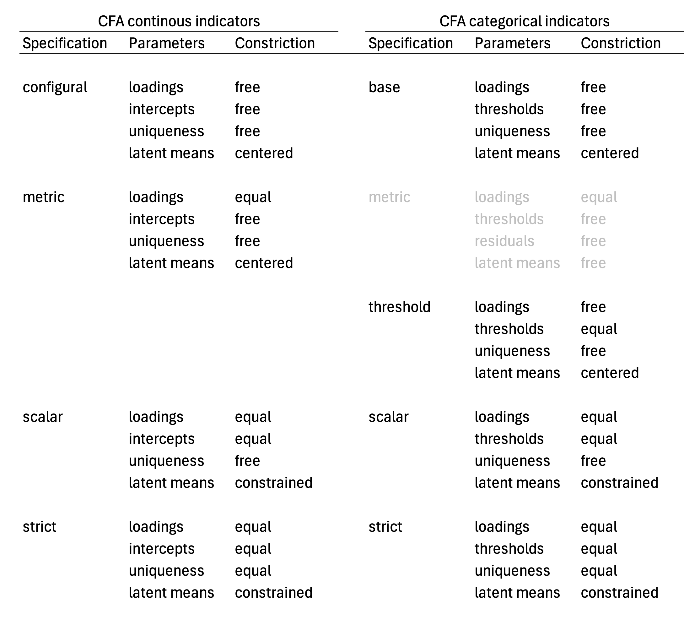
Figure 1: response model parameters being held equal in each model specification.

The present table is a rough summary of the different response model parameters that are held equal among groups, to specify each model solution. For example, in Wu & Estabrook (2016) the configural model specification for the CFA with ordinal indicators consists of a model where thresholds are held equal among groups. This is the baseline model from which model comparisons can be made in contrast to scalar and strict solutions of the GRM model. However, the configural model has more constraints than solely common thresholds, this includes factor means constrained to zero (i.e., centered) and factor variances fix to 1 on all groups (see Svetina et al., 2020). Additionally, Tse et al. (2024) discussess alternative model specification for the configural solution, using the theta parametrization in which factor loadings are held common between groups, and threshols are held common for marker indicators. In the present guidelines we will review these model specifications in more detail in section 4, following Svetina et al. (2020) and Wu & Estabrook (2016).

It should be clear that model specifications propose for CFA with continous indicators are not equivalent for other response models. The weak invariance (e.g., Dimitrov, 2010) or metric invariance model specification (Wu & Estabrook, 2016), where common factor loadings are held equal across groups, do not reach a model specification that holds the same interpretation of traditional CFA, for CFA with ordinal indicators (Wu & Estabrook, 2016; Svetina, et al. 2020; Tse, et al, 2024). A similar observation can be done for the assumed interpretation of the metric model specification of latent class models (e.g., Hooghe & Oser, 2015; Hooghe et al. 2016), which is an special case of a non-invariant solution (Masyn, 2017), and doesn’t hold the same interpretation of the random term across groups, the configuration of the laten classess (Torres Irribarra, et al., 2021). If invariance holds, the purpose is to assert that group differences are on the random term of the response model (i.e., factors, latent means, latent classes); in contrast, if the model specification doesn’t provide group differences estimates on the same scale, then subtantive conclusions are not tenable, because these do not have a common meaning between groups. In summary, the interpretation one can hold over response models fitted between groups with varying equality constrains among groups are not equivalent between response models.

In the following section (section 2) we will describe what are partially invariant solutions.

References

Carrasco, D., Irribarra, D. T., & González, J. (2022). Continuation Ratio Model for Polytomous Items Under Complex Sampling Design. In Quantitative Psychology (pp. 95–110). https://doi.org/10.1007/978-3-031-04572-1_8

Dimitrov, D. M. (2010). Testing for Factorial Invariance in the Context of Construct Validation. Measurement and Evaluation in Counseling and Development, 43, 121–149. https://doi.org/10.1177/0748175610373459

Bovaird, J. A., & Koziol, N. A. (2012). Measurement Models for Ordered-Categorical Indicators. In R. H. Hoyle (Ed.), Handbook of Structural Equation Modeling (pp. 495–511). Guilford Press.

Grimm, K. J., & Liu, Y. (2016). Residual Structures in Growth Models With Ordinal Outcomes. Structural Equation Modeling, 23(3), 466–475. https://doi.org/10.1080/10705511.2015.1103192

Hooghe, M., & Oser, J. (2015). The rise of engaged citizenship: The evolution of citizenship norms among adolescents in 21 countries between 1999 and 2009. International Journal of Comparative Sociology, 56(1), 29–52. https://doi.org/10.1177/0020715215578488.

Hooghe, M., Oser, J., & Marien, S. (2016). A comparative analysis of ‘good citizenship’: A latent class analysis of adolescents’ citizenship norms in 38 countries. International Political Science Review, 37(1), 115–129. https://doi.org/10.1177/0192512114541562.

Kline, R. B. (2023). Principles and Practice of Structural Equation Modeling (5th ed.). Guilford Press.

Masters, G. N. (1982). A rasch model for partial credit scoring. Psychometrika, 47(2), 149–174. https://doi.org/10.1007/BF02296272

Masyn, K. E. (2017). Measurement Invariance and Differential Item Functioning in Latent Class Analysis With Stepwise Multiple Indicator Multiple Cause Modeling. Structural Equation Modeling: A Multidisciplinary Journal, 24(2), 180–197. https://doi.org/10.1080/10705511.2016.1254049

Samejima, F. (1968). Estimation of latent Ability using a response pattern of graded scores. ETS Research Bulletin Series, 1968(1), i–169. https://doi.org/10.1002/j.2333-8504.1968.tb00153.x

Samejima, F. (2016). Graded Response Models. In W. J. van der Linden (Ed.), Handbook of Item Response Theory. Volume One. Models (pp. 95–107). CRC Press. https://doi.org/10.1201/9781315374512-16

Torres Irribarra, D. (2021). A Pragmatic Perspective of Measurement. Springer International Publishing. https://doi.org/10.1007/978-3-030-74025-2

Torres Irribarra, D., & Carrasco, D. (2021). Profiles of Good Citizenship. In E. Treviño, D. Carrasco, E. Claes, & K. J. Kennedy (Eds.), Good Citizenship for the Next Generation. A Global Perspective Using IEA ICCS 2016 Data (pp. 33–50). Springer International Publishing. https://doi.org/10.1007/978-3-030-75746-5_3

Tse, W. W. Y., Lai, M. H. C., & Zhang, Y. (2024). Does strict invariance matter? Valid group mean comparisons with ordered-categorical items. Behavior Research Methods, 56(4), 3117–3139. https://doi.org/10.3758/s13428-023-02247-6

Wang, J., & Wang, X. (2020). Confirmatory Factor Analysis. In Structural Equation Modeling: Applications Using Mplus (pp. 33–117). John Wiley & Sons, Inc. https://doi.org/10.4324/9781315832746-25

Wu, H., & Estabrook, R. (2016). Identification of Confirmatory Factor Analysis Models of Different Levels of Invariance for Ordered Categorical Outcomes. Psychometrika, 81(4), 1014–1045. https://doi.org/10.1007/s11336-016-9506-0