# -----------------------------------------------
# install rd3c3
# -----------------------------------------------

devtools::install_github(
  'dacarras/rd3c3',
  force = TRUE
)5 Applied Examples
5.1 Summary
- We use data from TIMSS 2019, from the student background questionnaire.
- In particular we are using student responses to the items of the scale “Sense of School Belonging”, from Chile and England.
- The data file includes 4115 students from Chile, and 3365 students from England, from 8th grade
- We are using a tailor-made data file where we include specific clustering and survey design variables:
- id_i = unique id number for students
- id_j = unique id number for schools
- id_s = unique id number for stratification factors (i.e., JKZONES)
- id_k = unique id number for country samples
- ws = scale survey weights to a constant of 1000
data_ex1.rds
- To install the library, a user can use the following code, to download the development version of the library:
- We include three applied examples:
- Invariance Analysis
- Model based invariance analysis
- Alignment method analsyis
- Item report analysis
- The item report analysis includes a larger set of analysis, besides Model based invariance analysis and Alignment method analsyis, such as item descriptives, missing data analysis, parallel analysis and reliability analysis among others.
- Invariance Analysis
5.2 Invariance analysis
5.2.1 Model based invariance analysis
Model based invariance analysis includes five model specifications:
pooled is a graded response model with probit link, including survey design variables (i.e., stratification factors, primary sampling unit and student survey weights) (e.g., Stapleton, 2013). Pooled a single measurement model, fitted onto pooled sample of cases were sampling weights have been scale to a common constant so including countries contributes equally to estimates (Gonzalez, 2012).
strict is a multigroup graded response model, where all response model parameters are held equal between compared groups, beside latent means for groups (Tse et al., 2024), while including the scale factors as part of the model.
scalar is a multigroup graded response model, where all response model parameters are held equal among groups, with the exemption of scale factors. It follows model specifications described in Svetina et al. (2020, proposition 7), where scale factors are fix to one for the reference group, and let to vary free on the rest of the groups in the comparison.
threshold is a multigroup graded response model, where thresholds are held common among the compared countries (i.e., threshold invariance). Is the baseline model for a model building sequence for assessing model-based measurement invariance (Wu & Estabrook, 2016). It follows model specifications described in Svetina et al. (2020, proposition 4).
configural is a multigroup graded response model, where all measurement model parameters are freely estimated among the compare groups, while holding latent factor means fix to zero, and factor variances fixed to one across groups.
Simulations studies from Rutkowski & Svetina (2017) with the graded response model with probit link and a larger amount of compare groups (e.g., 10, 20) suggest that RMSEA < .055 serves as a rule of thumb to select well-fitting measurement models with invariant parameters among compared groups.
To fit the following models we use as inputs:
- data_responses
data_ex1.rds - scale_info =
guideline_scale_info_example.xlsx - scale_id = 1
- and is using the functions:
rd3c3::fit_grm2for the pooled modelrd3c3::fit_grm2_m01_strictfor the strict modelrd3c3::fit_grm2_m02_scalarfor the scalar modelrd3c3::fit_grm2_m03_thresholdfor the threshold modelrd3c3::fit_grm2_m04_configfor the base model (i.e., descriptive model)
In the following section we include code (folded) to produce the invariance model fit indexes table (see Table 1).
Code
#------------------------------------------------------------------------------
# define objects
#------------------------------------------------------------------------------

# -----------------------------------------------
# scale id
# -----------------------------------------------

rd3c3::silent(library(dplyr))

# -----------------------------------------------
# scale id
# -----------------------------------------------

scale_id <- 1

# -----------------------------------------------
# scales info
# -----------------------------------------------

scales_data <- readxl::read_xlsx(
               'guideline_scale_info_example.xlsx',
               sheet = 'scales_data'
               )

# -----------------------------------------------
# data file
# -----------------------------------------------

data_file <- scales_data %>%
dplyr::filter(scale_num == scale_id) %>%
dplyr::select(data_file) %>%
unique() %>%
dplyr::pull()

# -----------------------------------------------
# response matrix
# -----------------------------------------------

data_responses <- readRDS(data_file) %>%
mutate(grp = paste0(COUNTRY)) %>%
mutate(grp = as.numeric(as.factor(COUNTRY))) %>%
mutate(grp_name = paste0(COUNTRY))

#------------------------------------------------------------------------------
# response models
#------------------------------------------------------------------------------

# -----------------------------------------------
# most centered
# -----------------------------------------------

grp_centered <- 'CHL'

# -----------------------------------------------
# pooled
# -----------------------------------------------

inv_0 <- rd3c3::silent(
             rd3c3::fit_grm2(
           data = data_responses,
           scale_num  = scale_id,
             scale_info = scales_data
              )
             )

# -----------------------------------------------
# strict
# -----------------------------------------------

inv_1 <- rd3c3::silent(
           rd3c3::fit_grm2_m01_strict(
           data = data_responses,
           scale_num = scale_id,
           scale_info = scales_data,
           grp_var = 'id_k',
           grp_txt = 'grp_name',
           grp_ref = grp_centered
           )
           )

# -----------------------------------------------
# scalar
# -----------------------------------------------

inv_2 <- rd3c3::silent(
           rd3c3::fit_grm2_m02_scalar(
           data = data_responses,
           scale_num = scale_id,
           scale_info = scales_data,
           grp_var = 'id_k',
           grp_txt = 'grp_name',
           grp_ref = grp_centered
           )
           )

# -----------------------------------------------
# threshold
# -----------------------------------------------

inv_3 <- rd3c3::silent(
           rd3c3::fit_grm2_m03_threshold(
           data = data_responses,
           scale_num = scale_id,
           scale_info = scales_data,
           grp_var = 'id_k',
           grp_txt = 'grp_name',
           grp_ref = grp_centered
           )
           )

# -----------------------------------------------
# configural
# -----------------------------------------------

inv_4 <- rd3c3::silent(
           rd3c3::fit_grm2_m04_config(
           data = data_responses,
           scale_num = scale_id,
           scale_info = scales_data,
           grp_var = 'id_k',
           grp_txt = 'grp_name',
           grp_ref = grp_centered
           )
           )

# -----------------------------------------------
# retrieve fit indexes per model
# -----------------------------------------------

fit_0 <- rd3c3::get_inv_fit(inv_0, model_name = 'pooled')
fit_1 <- rd3c3::get_inv_fit(inv_1, model_name = 'strict')
fit_2 <- rd3c3::get_inv_fit(inv_2, model_name = 'scalar')
fit_3 <- rd3c3::get_inv_fit(inv_3, model_name = 'threshold')
fit_4 <- rd3c3::get_inv_fit(inv_4, model_name = 'configural')

# -----------------------------------------------
# general table
# -----------------------------------------------

fit_table <- dplyr::bind_rows(
             dplyr::select(fit_0, model, RMSEA, CFI, TLI, SRMR, x2, df, p_val),
             dplyr::select(fit_1, model, RMSEA, CFI, TLI, SRMR, x2, df, p_val),
             dplyr::select(fit_2, model, RMSEA, CFI, TLI, SRMR, x2, df, p_val),
             dplyr::select(fit_3, model, RMSEA, CFI, TLI, SRMR, x2, df, p_val),
             dplyr::select(fit_4, model, RMSEA, CFI, TLI, SRMR, x2, df, p_val)
             )


# -----------------------------------------------
# model fit
# -----------------------------------------------

fit_table %>%
knitr::kable(.,
  digits = c(0,3,2,2,2,2,0,2),
    caption = 'Table 1: invariance model fit indexes between compared groups'
)| model | RMSEA | CFI | TLI | SRMR | x2 | df | p_val |
|---|---|---|---|---|---|---|---|
| pooled | 0.034 | 1.00 | 1.00 | 0.01 | 18.61 | 2 | 0 |
| strict | 0.042 | 0.99 | 1.00 | 0.02 | 112.97 | 15 | 0 |
| scalar | 0.027 | 1.00 | 1.00 | 0.01 | 40.66 | 11 | 0 |
| threshold | 0.032 | 1.00 | 1.00 | 0.01 | 37.18 | 8 | 0 |
| configural | 0.044 | 1.00 | 0.99 | 0.01 | 31.78 | 4 | 0 |
Note: pooled = is the measurement model fitted onto the pooled sample. strict = is a multigroup measurement model with common thresholds, common loadings, and a common scale. This latent variable model suffices mean score comparisons (Tse et al., 2024). scalar = is a multigroup measurement model with common thresholds, common loadings, and free scales for each item. This model supports latent mean comparisons (Tse et al., 2024). threshold = is a multigroup measurement model with common thresholds. configural = is a multigroup descriptive model where all measurement model parameter are free to vary. Metric model specification is not identified under the graded response models (Wu & Estabrook, 2016), thus metric specifications are not included. A RMSEA of .055 or less has been found to be good threshold for fit for graded response models with many groups of 10 or 20 compared groups (see Rutkowski & Svetina, 2017).
5.2.2 Alignment
The alignment method is optimizing for the least discrepant measurement model parameters among the compared groups. Is fitting a graded response model with probit link, and using the most optimal group as a reference. We are using the statement ALIGNMENT = FIXED(*); within Mplus for these purposes. We rely on the Measurement invariance explorer (https://github.com/MaksimRudnev/MIE.package) to retrieve aligment results.
The following code (folded) is used as inputs:
- data_responses
data_ex1.rds - scale_info =
guideline_scale_info_example.xlsx - scale_id = 1
- and is using the function
rd3c3::fit_grm2_align_wlsmv()to run an alignment method analysis
Code
#------------------------------------------------------------------------------
# define objects
#------------------------------------------------------------------------------

# -----------------------------------------------
# scale id
# -----------------------------------------------

rd3c3::silent(library(dplyr))

# -----------------------------------------------
# scale id
# -----------------------------------------------

scale_id <- 1

# -----------------------------------------------
# scales info
# -----------------------------------------------

scales_data <- readxl::read_xlsx(
               'guideline_scale_info_example.xlsx',
               sheet = 'scales_data'
               )

# -----------------------------------------------
# data file
# -----------------------------------------------

data_file <- scales_data %>%
dplyr::filter(scale_num == scale_id) %>%
dplyr::select(data_file) %>%
unique() %>%
dplyr::pull()

# -----------------------------------------------
# response matrix
# -----------------------------------------------

data_responses <- readRDS(data_file) %>%
mutate(grp = paste0(COUNTRY)) %>%
mutate(grp = as.numeric(as.factor(COUNTRY))) %>%
mutate(grp_name = paste0(COUNTRY))

#------------------------------------------------------------------------------
# alignment
#------------------------------------------------------------------------------

# -----------------------------------------------
# aligned
# -----------------------------------------------


fitted_align <- rd3c3::silent(
rd3c3::fit_grm2_align_wlsmv(
data = data_responses,
scale_num = scale_id,
scale_info = scales_data)
)

# -----------------------------------------------
# retrieve output
# -----------------------------------------------

scale_file <- scales_data %>%
dplyr::filter(scale_num == scale_id) %>%
dplyr::select(mplus_file) %>%
unique() %>%
dplyr::pull()


alignment_out <- MIE::extractAlignment(paste0(scale_file,'_align.out'), silent = TRUE)

# -----------------------------------------------
# display
# -----------------------------------------------

alignment_table <- alignment_out$summary %>%
                   tibble::rownames_to_column("terms") %>%
                   tibble::as_tibble() %>%
                   rename(
                   term        = 1,
                   a_par       = 2,
                   R2          = 3,
                   n_inv       = 4,
                   n_dis       = 5,
                   inv_grp     = 6,
                   dis_grp     = 7
                   ) %>%
                   mutate(type = case_when(
                   stringr::str_detect(term, 'Threshold') ~ 'tau',
                   stringr::str_detect(term, 'Loadings')  ~ 'lambda'
                   )) %>%
                   mutate(term = stringr::str_replace(term, '\\$', '_')) %>%
                   mutate(term = stringr::str_replace(term, 'Threshold', '')) %>%
                   mutate(term = stringr::str_replace(term, 'Loadings', '')) %>%
                   mutate(term = stringr::str_replace(term, 'ETA by ', '')) %>%
                   dplyr::select(
                   type, term, a_par, R2, n_inv, n_dis, inv_grp, dis_grp)

# -----------------------------------------------
# display
# -----------------------------------------------

alignment_table %>%
knitr::kable(.,
  digits = 2,
    caption = 'Table 2: alignment comparisons'
)| type | term | a_par | R2 | n_inv | n_dis | inv_grp | dis_grp |
|---|---|---|---|---|---|---|---|
| tau | I01_1 | NA | NA | 0 | 2 | 18 11 | |
| tau | I01_2 | NA | NA | 0 | 2 | 18 11 | |
| tau | I01_3 | 0.73 | 1.00 | 2 | 0 | 11 18 | |
| tau | I02_1 | -1.89 | 0.94 | 2 | 0 | 11 18 | |
| tau | I02_2 | -1.09 | 0.00 | 2 | 0 | 11 18 | |
| tau | I02_3 | NA | NA | 0 | 2 | 18 11 | |
| tau | I03_1 | -1.73 | 0.83 | 2 | 0 | 11 18 | |
| tau | I03_2 | -1.00 | 0.91 | 2 | 0 | 11 18 | |
| tau | I03_3 | 0.20 | 0.85 | 2 | 0 | 11 18 | |
| tau | I05_1 | -1.64 | 0.88 | 2 | 0 | 11 18 | |
| tau | I05_2 | -0.97 | 0.01 | 2 | 0 | 11 18 | |
| tau | I05_3 | 0.23 | 0.93 | 2 | 0 | 11 18 | |
| lambda | I01 | 0.72 | 0.00 | 2 | 0 | 11 18 | |
| lambda | I02 | 0.77 | 0.20 | 2 | 0 | 11 18 | |
| lambda | I03 | 0.84 | 0.26 | 2 | 0 | 11 18 | |
| lambda | I05 | 0.80 | 0.00 | 2 | 0 | 11 18 |
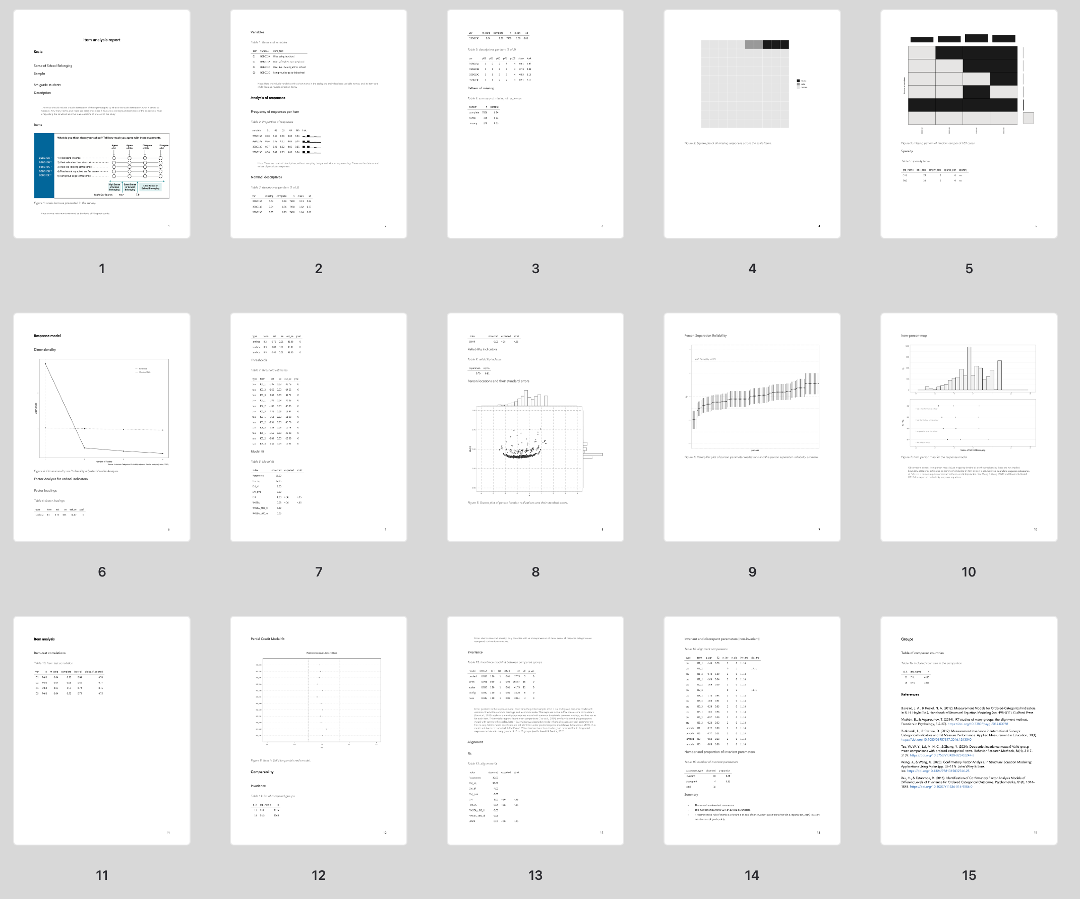
5.3 Item report analysis
In the following section we include a template example, to produce item analysis reports. This template includes:
- Scale description
- a presentation of the name of the collection of items (i.e., the scale name)
- a presentation of items as these where presented to the participants
- a table with the item text, with the public data file names, and the shortened variable names
- Analysis of responses
- descriptives
- missing data descriptives
- Response model
- dimensionality analysis via parallel analysis for ordinal indicators (Lubbe, 2019)
- response model parameters for a graded response model
- reliability analysis
- item person maps
- Item analysis
- item test correlation
- item fit based on partial credit model
- Comparability
- model based measurement invariance
- alignment analysis of GRM among groups
The following figure depicts an overview of the generated report.
To produce this examplary report the user needs as inputs:
- data_responses
data_ex1.rds - scale_info =
guideline_scale_info_example.xlsx - scale_id = 1
- the template
guideline_item_report_example.rmd- and the word template
report_template.docx
- and the word template
The end product of this procedure can be inspected in the following file guideline_item_report_example.docx
5.4 Additional examples
The current examples are just toy examples, to illustrate the basic capabilities of the library. We include two other data response files. One example with three countries, where is possible to see that three countries do not obtain strict invariance (example with “Sense of School Belonging” for three countries). And a third example of a template-based workflow, where we procede with a full fledge item analysis report including all participating countries (example with the “Bullying Scale” for all participating countries).
- Example with “Sense of School Belonging” for three countries
- data:
data_example.rds - code template:
template_example_2.rmd- word template:
report_template.docx
- word template:
- resulting report:
template_example_2.docx
- data:
- Example with “Bullying Scale” for all participating countries
- data:
survey_1_g8.rds - code template:
template_example_3.rmd- word template:
report_template.docx
- word template:
- resulting report
template_example_3.docx.
- data:
All example files can be downloaded from the following link.
5.5 References
Gonzalez, E. J. (2012). Rescaling sampling weights and selecting mini-samples from large-scale assessment databases. IERI Monograph Series Issues and Methodologies in Large-Scale Assessments, 5, 115–134.
Tse, W. W. Y., Lai, M. H. C., & Zhang, Y. (2024). Does strict invariance matter? Valid group mean comparisons with ordered-categorical items. Behavior Research Methods, 56(4), 3117–3139. https://doi.org/10.3758/s13428-023-02247-6
Stapleton, L. M. (2013). Incorporating Sampling Weights into Single- and Multilevel Analyses. In L. Rutkowski, M. von Davier, & D. Rutkowski (Eds.), Handbook of International Large scale Assessment: background, technical issues, and methods of data analysis (pp. 363–388). Chapman and Hall/CRC.
Svetina, D., Rutkowski, L., & Rutkowski, D. (2020). Multiple-Group Invariance with Categorical Outcomes Using Updated Guidelines: An Illustration Using Mplus and the lavaan/semTools Packages. Structural Equation Modeling: A Multidisciplinary Journal, 27(1), 111–130. https://doi.org/10.1080/10705511.2019.1602776
Wu, M., Tam, H. P., & Jen, T.-H. (2016). Educational Measurement for Applied Researchers. Springer Singapore. https://doi.org/10.1007/978-981-10-3302-5
Rutkowski, L., & Svetina, D. (2017). Measurement Invariance in International Surveys: Categorical Indicators and Fit Measure Performance. Applied Measurement in Education, 30(1). https://doi.org/10.1080/08957347.2016.1243540